INTRODUCTION TO MATLAB

Chapter 11
Interpolation and Extrapolation

Since Matlab only represents functions as arrays of values a common problem that comes
up is finding function values at points not in the arrays. Finding function values between
data points in the array is called interpolation, finding function values beyond the endpoints
of the array is called extrapolation. A common way to do both is to use nearby function
values to define a polynomial approximation to the function that is pretty good over a small
region. Both linear and quadratic function approximations will be discussed here.

11.1 Linear Interpolation and Extrapolation
A linear approximation can be obtained with just two data points, say (x₁, y₁) and (x₂, y₂).
You learned a long time ago that two points define a line and that the two-point formula
for a line is

This formula can be used between any two data points to linearly interpolate. For example,
if x in this formula is half-way between x₁ and x₂ at x = (x₁+x₂)/2 then it is easy to show
that linear interpolation gives the obvious result y = (y₁ + y₂)/2.

But you must be careful when using this method that your points are close enough
together to give good values. In Fig. 11.1, for instance, the linear approximation to the
curved function represented by the dashed line "a" is pretty poor because the points x = 0
and x = 1 on which this line is based are just too far apart. Adding a point in between at
x = 0.5 gets us the two-segment approximation "c" which is quite a bit better. Notice also
that line "b" is a pretty good approximation because the function doesn't curve much.

This linear formula can also be used to extrapolate. A common way extrapolation is
often used is to find just one more function value beyond the end of a set of function pairs
equally spaced in x. If the last two function values in the array are f_N-1 and f_N, it is easy
to show that the formula above gives the simple rule

which was used in the Matlab code in Sec. 10.1

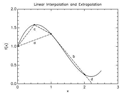
Figure 11.1 Linear interpolation only works well over intervals
where the function is straight.
You must be careful here as well: segment "d" in Fig. 11.1 is the linear extrapolation of
segment "b", but because the function starts to curve again "d" is a lousy approximation
unless x is quite close to x = 2.

11.2 Quadratic Interpolation and Extrapolation
Quadratic interpolation and extrapolation are more accurate than linear because the
quadratic polynomial ax² + bx + c can more easily t curved functions than the linear
polynomial ax + b. Consider Fig. 11.2. It shows two quadratic fits to the curved function.
The one marked "a" just uses the points x = 0, 1, 2 and is not very accurate because these
points are too far apart. But the approximation using x = 0, 0.5, 1, marked "b", is really
quite good, much better than a two-segment linear t using the same three points would
be.

Unfortunately, the formulas for quadratic fitting are more difficult to derive. (The
Lagrange interpolation formulas, which you can find in most elementary numerical analysis
books, give these formulas.) But for equally spaced data in x, Taylor's theorem, coupled with
the approximations to the first and second derivatives discussed in the section on numerical
derivatives, make it easy to derive and use quadratic interpolation and extrapolation. We
want to do it this way because it uses the approximate derivative formulas we used in
Sec. and illustrates a technique which is widely used in numerical analysis.

You may recall Taylor's theorem that an approximation to the function f(x) near the
point x = a is given by

Let's use this approximation (ignoring all terms beyond the quadratic term in (x - a))
near a point (x_n, f_n ) in an array of equally spaced x values. The grid spacing in x is h.

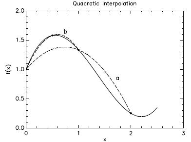
Figure 11.2 Quadratic interpolation follows the curves better if
the curvature doesn't change sign.

An approximation to Taylor's theorem that uses numerical derivatives in this array is then
given by

This formula is very useful for getting function values that aren't in the array. For instance,
it is easy to use this formula to obtain the interpolation approximation to f(x_n + h/2)

and also to find the quadratic extrapolation rule

11.3 Interpolating With polyfit and polyval
You can also use Matlab's polynomial commands (which you learned about in Chapter 8)
to build an interpolating polynomial. Here is an example of how to use them to find a
5th-order polynomial t to a crude representation of the sine function.

Example 11.3a (ch11ex3a.m) % Example 11.3a (Physics 330) clear, close all, % make the crude data set with dx too big for % good accuracy dx=pi/5, x=0:dx:2*pi, y=sin(x), % make a 5th order polynomial fit to this data p=polyfit(x,y,5), % make a fine x-grid xi=0:dx/20:2*pi, % evaluate the fitting polynomial on the fine grid yi=polyval(p,xi), % and display the fit, the data, and the exact sine function plot(x,y,'b*',xi,yi,'r-',xi,sin(xi),'c-') legend('Data','Fit','Exact sine function') % display the difference between the polynomial fit and % the exact sine function figure plot(xi,yi-sin(xi),'b-') title('Error in fit')

11.4 Matlab Commands Interp1 and Interp2
Matlab has its own interpolation routine interp1 which does the things discussed in this
section automatically. Suppose you have a set of data points {x, y} and you have a different
set of x-values {x_i} for which you want to find the corresponding {y_i} values by interpolating
in the {x, y} data set. You simply use any one of these three forms of the interp1 command:
yi=interp1(x,y,xi,'linear')
yi=interp1(x,y,xi,'cubic')
yi=interp1(x,y,xi,'spline')

Here is an example of how each of these three types of interpolation works on a crude
data set representing the sine function.

Example 11.4a (ch11ex4a.m) % Example 11.4a (Physics 330) clear, close all, % make the crude data set with dx too big for % good accuracy dx=pi/5, x=0:dx:2*pi, y=sin(x), % make a fine x-grid xi=0:dx/20:2*pi, % interpolate on the coarse grid to % obtain the fine yi values % linear interpolation yi=interp1(x,y,xi,'linear'), % plot the data and the interpolation plot(x,y,'b*',xi,yi,'r-') title('Linear Interpolation') % cubic interpolation yi=interp1(x,y,xi,'cubic'), % plot the data and the interpolation figure plot(x,y,'b*',xi,yi,'r-') title('Cubic Interpolation') % spline interpolation yi=interp1(x,y,xi,'spline'), % plot the data and the interpolation figure plot(x,y,'b*',xi,yi,'r-') title('Spline Interpolation')

Matlab also knows how to do 2-dimensional interpolation on a data set of {x, y, z} to
find approximate values of z(x, y) at points {x_i, y_i} which don't lie on the data points {x, y}.
You could use any of the following
zi = interp2(x,y,z,xi,yi,'linear')
zi = interp2(x,y,z,xi,yi,'cubic')
zi = interp2(x,y,z,xi,yi,'spline')

This will work fine for 1-dimensional data pairs {x_i, y_i}, but you might want to do this
interpolation for a whole bunch of points over a 2-d plane, then make a surface plot of
the interpolated function z(x, y). Here's some code to do this and compare these three
interpolation methods (linear, cubic, and spline).

Example 11.4b (ch11ex4b.m) % Example 11.4b (Physics 330) clear, close all, x=-3:.4:3, y=x, % build the full 2-d grid for the crude x and y data % and make a surface plot [X,Y]=meshgrid(x,y), Z=cos((X.^2+Y.^2)/2), surf(X,Y,Z), title('Crude Data') %********************************************************* % now make a finer 2-d grid, interpolate linearly to % build a finer z(x,y) and surface plot it. % Note that because the interpolation is linear the mesh is finer % but the crude corners are still there %********************************************************* xf=-3:.1:3, yf=xf, [XF,YF]=meshgrid(xf,yf), ZF=interp2(X,Y,Z,XF,YF,'linear'), figure surf(XF,YF,ZF), title('Linear Interpolation') %********************************************************* % Now use cubic interpolation to round the corners. Note that there is % still trouble near the edge because these points only have data on one % side to work with, so interpolation doesn't work very well %********************************************************* ZF=interp2(X,Y,Z,XF,YF,'cubic'), figure surf(XF,YF,ZF), title('Cubic Interpolation') %********************************************************* % Now use spline interpolation to also round the corners and see how % it is different from cubic. You should notice that it looks better, % especially near the edges. Spline interpolation is often the % best. %********************************************************* ZF=interp2(X,Y,Z,XF,YF,'spline'), figure surf(XF,YF,ZF), title('Spline Interpolation')

For more detail see Mastering Matlab 6, Chapter 19.