Equilibrium Values and their Stability for First-Order Non-Linear DDS

In order to use x(1) as the next input value, we have to transfer its value from the vertical to the
horizontal axis. We could just read it off, and then mark the appropriate value on the horizontal
axis. Alternatively, we can use the 45° line (where input and output values are identical) to assist
with the transfer. To make the output value into an input value, we draw a horizontal line from
x(1) to the 45° line, then a vertical line down to the horizontal axis (thick lines in the graph
below). This transforms the value of x(1) from output to input value.

We repeat this process, now starting with x(1) , until we have transferred the value of x(2) to the
horizontal axis. You may notice that each step creates a number of lines, parts of which are drawn
twice. Those segments, as well as the initial vertical line, are shown as thin lines in the next graph.
All other segments are drawn as thick lines; they constitute the Cobb-web diagram and are the
only ones usually drawn.

Such a Cobb-web diagram can be created with the palette function MapIt. The function MapIt
needs as its entries the following:

?MapIt
The function MapIt[{func, x}, xinit, n, {xmin, xmax}, focus,
percent] displays n iterations of the function func expressed in
terms of x. The iteration starts at x = xinit and is displayed
for x-values from xmin to xmax. When zooming in, the graph is
centered at x = focus. The value of percent determines the amount
of zooming: For 0 < percent < 1, we zoom in, for percent > 1, we
zoom out.

Let’s look at the different entries one by one for our example. The model function is f (x) = 5x² ,
thus func = 5x² , and the variable used is x. The initial value is xinit = 0.1. To see 5 iterations, we
set n = 5. The table of values (= A1) and the previous graph indicate that choosing {0, 0.12} as the
range for the horizontal axis will show all intermediate steps. We can choose the midpoint on the
horizontal axis as the center point, i.e., focus = (0 + 0.12)/2 = 0.06, and no zooming, i.e., percent
= 1. This leads to the following use of MapIt:

We can see that the zig-zag line moves toward the equilibrium point (0,0) (input value =
equilibrium value = 0). This shows that if we start with an initial value slightly above the
equilibrium value, then the sequence of values converges towards the equilibrium value. Next we
create a Cobb-web diagram for an initial value slightly below the equilibrium value by adjusting
the values of xinit, xmin, xmax and focus in the function MapIt. We can choose xinit = -0.1,
{xmin, xmax} = {-0.12, 0.02} (equilibrium value at 0), and focus = -0.05.

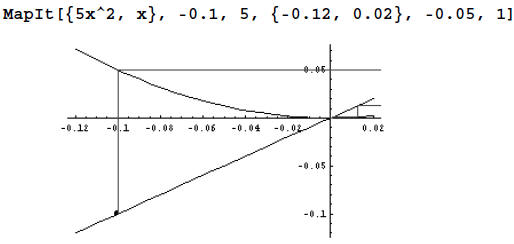
You may be a bit surprised by this graph. However, a close look at the values in the column for
A2 (in the previous table) shows that x(2) = 0.05. All later values in the sequence are smaller.
Thus, we should use {xmin, xmax} = {-0.12, 0.07} and focus = (-0.12+0.07)/2 = -0.025 to see
the full Cobb-web diagram. (Alternatively, you can choose focus = 0 for simplicity).

Since the sequence values approach the equilibrium value whether x(0) is slightly above or below
the equilibrium value, we conclude that x = 0 is a stable equilibrium.

The Cobb-web diagram looks quite different from the graphs we have seen before. Note that the
axes display input and output values, but not time. Thus, the Cobb-web diagram visualizes the
iterative model equation (where x(n+1) is a function of (x(n)), whereas the graphs created by
ListGraph visualize the model solution (where x(n) is a function of n).

Below is an illustration on how the two types of graphs relate to each other. We start by creating
a Cobb-web diagram. Below this graph we put another set of horizontal and vertical axes. On the
horizontal axis we mark x(n), on the vertical axis we mark the time n. Now we extend the vertical
lines of the Cobb-web graph downwards (through the value x(k)) until we reach time k.

If we now take the lower part of this graph and rotate it by 90° , then we get a graph
corresponding to the explicit solution, the type of graph that is produced by ListGraph.

Let's now check the second equilibrium with this new method, using initial values
x(0) = 0.1. and x(0) = 0.3. We have already seen the Cobb-web diagram for x(0) = 0.1 and know
that the values tend toward 0, not 0.2. This indicates that the equilibrium cannot be stable. Let's
see what happens for x(0) = 0.3. (Note that focus was not chosen to be the midpoint.)

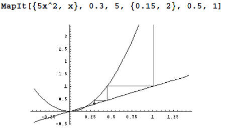
The graph shows that for a initial value slightly above the equilibrium value, the sequence again
moves away from the equilibrium value of 0.2. This makes an unstable equilibrium.

Activity 6.6.2 For the DDS given below, determine the stability of the equilibrium value(s) in two different ways, by using 1) the functions IteratedValueSeq and ListGraph, and 2) the function MapIt. (Note: These are the DDS from Activity 6.6.1)

You can see a live animation of the Cobb-web diagram by using the function LiveMap. LiveMap
uses entries very similar to the ones used in MapIt.

?LiveMap
The function LiveMap[{func, x}, xinit, n, {xmin, xmax},
{ymin, ymax}]creates the graphics for an animation of n
iterations of the function func expressed in terms of x.
The iteration starts at x = xinit and is displayed for
input values from xmin to xmax and output values from ymin
to ymax.

MapIt and LiveMap only differ in the last two entries. In addition to specifying the range of
display on the horizontal axis, we also indicate the range of display for the vertical axis. LiveMap
creates a sequence of graphs, each displayed in a separate cell. Double clicking the cell bracket
that encloses all of the graphs (2^nd bracket from the left) collapses the cells so that only the first
graph remains visible. Select Cell -> Animate Selected Graphics or use the shortcut Ctrl-Y to
start the animation. You can control the spead of the animation by using the video panel that
appears on the lower left corner of the notebook. To stop the animation temporarily, use the ||
button. To permanently stop the animation, click anywhere in the notebook outside the graph.