Sidebar Menu


College Algebra
13 Inverse Functions
Definition 13.1. Two functions f and g are said to be inverse
functions
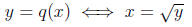
iff the graphs the equations y = f(x) and x = g(y) are the same, i.e. iff
y = f(x) ![]() x = g(y).
x = g(y).
We also say that g is the inverse of f and write
g = f -1.
Example 13.2. Since
the functions f(x) = 3x + 7 and g(y) = (y - 7)/3 are inverse functions.
Remark 13.3. Be careful not to confuse f(x)-1 and f -1(x).
For example,
if f(x) = 3x + 7, then
13.4. If f and g are inverse functions, then the range of
f is the domain of g
and the domain of f is the range of g. To decide if a function has an inverse
we apply the
| Horizontal Line Test. A function y = f(x) has an
inverse if and only if every horizontal line y = b intersects the graph in at most one point. Then the horizontal line y = b intersects the graph y = f(x) in the point P(f -1(b), b). |
13.5. A function f is said to be one-to-one iff

Saying that a function is one-to-one is just another way of saying its graph
satisfies the horizontal line test, i.e. that the function has an inverse. The
function f(x) = x2 is not one-to-one since f(3) = f(-3) but 3 ≠ -3.
Definition 13.6. A function f is said to be increasing iff
A function f is said to be decreasing iff

Theorem 13.7. If a function either increasing or decreasing it is one-to-one
and therefore has an inverse.
Proof. Assume f is increasing and that  . Then it is not the
case that  since that would imply
 and it is not the case
that  since that would imply
 . The only possibility us
that  .
.
Remark 13.8. Just because a function has an inverse
doesn't mean that we
can find a formula for the inverse. For example, the function f(x) = x5 + x
is increasing and therefore has an inverse f -1, but in graduate courses in
algebra it is proved that there is no elementary formula for f -1(y), i.e. there
is no expression for f -1(y) involving only the operations we have have defined
in these notes. Put another way, there is no nice formula for the solution of
the equation 3 = x5 + x.
Even if we can't find a formula for the inverse of a function, we can still
compute its value for any given input to any degree of accuracy with (say)
a computer. So we can give the inverse a name and compute with it using
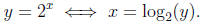
the rules of algebra. This is exactly what we shall do in Section 17. with the
exponential function
f(x) = 2x.
This function is increasing so has an inverse function. and the inverse func-
tion is denoted by  :
:
13.9. In Section 12.3 we said that, unless the contrary is stated, the domain
of a function f(x) which is defined by an expression in x is the set of x for
which the expression is meaningful. However, we may decide to restrict the
domain to a smaller set in order to define an inverse function. For example,
in Section 13.5 we saw that the function f(x) = x2 is not one-to-one since
f(3) = f(-3) and hence this function does not have an inverse function. But
we can define
q(x) = x2. x ≥ 0
so the domain is [0,∞). Then
so q(x) and  are inverse functions. (This device is used in trigonometry to
define the inverse trigonometric functions.) If we were to program a computer
to compute the function q(x), asking the computer to compute q(-3) would
produce an error message like \function undefined for this input".
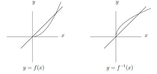
13.10. If the function f has an inverse, then the graph of the equation
y = f(x) is the same as the graph of the equation x = f -1(y). Of course
the graph of the equation y = f -1(x) is (usually) different. The graphs of
the equations y = f(x) and y = f -1(x) are obtained from
each other by
interchanging the x-axis and the y-axis, i.e. by reflecting in the line y = x.
14 Average Rate of Change
Definition 14.1. The average rate of change of the function f over the
interval [a, b] is the slope of the line joining the point (a, f(a)) to the
point
(b, f(b)). When y = f(x) the average rate of change is often written as
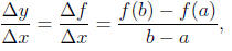
i.e. the average rate of change is the change Δy = f(b) -
f(a) in y divided
by the change Δx = b - a in x.
Example 14.2. The average rate of change of the function f(x) = x2 on
the interval [a, b] is
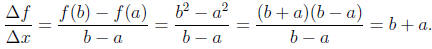
Note that the b-a in the denominator cancels out. To see
way this happens
we will repeat the calculation using the notation h = b - a = Δx so that
b = a + h. When we expand the numerator the terms which don't contain
an h cancel. Then the h in the denominator cancels with (some of) the h's
in the numerator as follows:

This cancellation will always happen when you are asked to
simplify an
average rate of change.
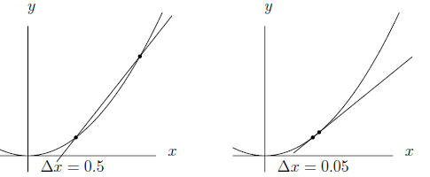
14.3. The average rate of change of a function f over the interval [a, b] is
undefined when a = b (zero divided by zero is nonsense) but for b very close
to a the average rate of change will usually be close to a number called the
instantaneous rate of change. This is the slope of the tangent line to the
graph y = f(x) at the point (a, f(a)).
In calculus the instantaneous rate of change is called the
derivative. In the
previous paragraph we saw that for the function f(x) = x2 the average rate
of change over the interval [a, b] is a+b. This is 2a+h where h =Δx = b-a.
The instantaneous rate of change at the point (a, f(a)) is 2a which is obtained
from the average rate of change by taking h = 0.
14.4. Suppose you are traveling from Madison to Milwaukee by automobile
via the interstate highway I-94. Your position is a function s = f(t) of the
time t. The value s is the number on the mile marker at the side of the
road. (Along much of the road there is a mile marker every tenth of a mile,
but imagine there is one every few feet.) The change Δs = f(t + Δt) - f(t)
is also the change in the odometer reading in your car. If the time interval
Δt is so short that your speed doesn't change much in the time interval, the
average rate of change Δs/ Δt is your speed as shown on the speedometer.
The speed is the instantaneous rate of change of the position.
15 Polynomials
15.1. For any graph the points where it intersects the x-axis are called the
x-intercepts and the points where it intersects the y-axis are called the y-
intercepts. The equation of the x-axis is y = 0 so we find
the x-intercepts
of the graph of an equation by plugging in y = 0 and solving for x. Similarly
the equation of the y-axis is x = 0 so we find the y-intercepts by plugging in
x = 0 and solving for y. If the graph is the graph of a function y = f(x),
then (assuming that 0 is in the domain) the y-intercept is the point (0, f(0)),
and the x-intercepts are the points (r, 0) such that f(r) = 0. The numbers
r such that f(r) = 0 are called the zeros (and sometimes also the roots) of
the function.
Definition 15.2. A polynomial is a function of form

where the exponents on x are nonnegative integers. A polynomial equation
is an equation of form

Its solutions are the zeros of the polynomial and are also called the roots of
the polynomial. When  ≠ 0 we say that the degree
of the polynomial is n.
≠ 0 we say that the degree
of the polynomial is n.
The constants  are called the coefficients. For any polynomial
f(0) =  (the constant term) so the y-intercept of the graph is the point

15.3. A polynomial of degree one (or zero) is called linear (since its graph
is a line), a polynomial of degree two is called quadratic, and a polynomial
of degree three is called cubic. In Paragraph 6.4 we used the notation
f(x) = mx + b (slope-intercept form) rather than
 for a
for a
linear function and in Theorem 11.2 we wrote the quadratic equation as
ax2 + bx + c = 0 rather than as  .
.
15.4. It is easy to graph a linear function: just find two points

and  on the graph and draw the line through them. It is also not
hard to graph a quadratic function f(x) = ax2 + bx + c. The graph is a
parabola which opens up (like y = x2) if a > 0 and down (like y = -x2)
if a < 0. By the Quadratic Formula in Theorem 11.2 the graph has two
x-intercepts if the discriminant b2 - 4ac is positive, one x-intercept if the
discriminant is zero, and no x-intercept if the discriminant is negative.
Remark 15.5. When a = 1 and b and c are integers we could
try to solve
the quadratic equation x2 + bx + c = 0 by factoring. If

(for all x) then

If we suspect that the roots are integers, we can try all possible ways of
factoring c. For example, to solve x2 - 5x + 6 = 0 we try
 ,
,
(-1,-6), (2, 3), (-2,-3). Only  gives
gives
 so
so
x2 - 5x + 6 = (x - 2)(x - 3)
and the solutions of x2 - 5x + 6 = 0 are x = 2 and x = 3. Of course, there
is usually no reason to suspect that the roots are integers so it is best to use
the Quadratic Formula (Theorem 11.2) to solve a quadratic equation.
15.6. A polynomial inequality like

is easy to solve if we can factor the left hand side. Then we can write it in
the form

On each of the intervals  the sign
of
the sign
of
the polynomial is constant so we can compute the sign by evaluating the
polynomial at some point in the interval. For example,
(x - 1)(x - 4)(x - 9) > 0
![]() x in (1, 4) ∪ [ (9,∞)
x in (1, 4) ∪ [ (9,∞)
and
(x - 1)(x - 4)(x - 9) ≥ 0 ![]() x in [1, 4] ∪ [ [9,∞)
x in [1, 4] ∪ [ [9,∞)
As a check we evaluate
at x = 0 in (-∞, 1) and get (0 - 1)(0 - 4)(0 - 9) = -36 < 0,
at x = 2 in (1, 4) and get (2 - 1)(2 - 4)(2 - 9) = 14 > 0,
at x = 5 in (4, 9) and get (5 - 1)(5 - 4)(5 - 9) = -16 < 0, and
at x = 10 in (9,∞) and get (10 - 1)(10 - 4)(10 - 9) = 54 > 0.
15.7. To graph a polynomial f(x) we use the following rules:
(i) The sign of the polynomial does not change between two
adjacent roots.
To determine this sign we can evaluate the polynomial at any number
in between.
(ii) If the polynomial can be factored so that

where  are the roots, then between each pair of
roots  the graph reverses direction exactly once, i.e. either the
function value f(x) increases on some interval
 and then decreases
on the interval  or it decreases on some
interval and then
or it decreases on some
interval and then
increases on the interval
(iii) The absolute value of f(x) is large when the absolute value of x is large.
Whether f(x) is large positive or large negative depends only on the
sign of the coefficient of xn (where n is the degree) and on whether n
is odd or even.
In calculus you will learn how to determine on which intervals the function
is increasing and you will learn enough to understand why (ii) is true.
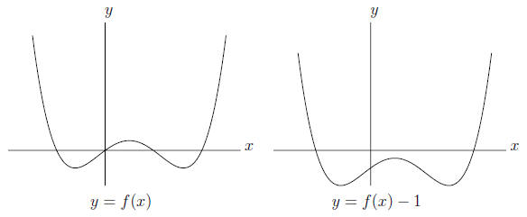
Below we have graphed the polynomial
f(x) = x4 - 2x3 - x2 + 2x = (x + 1)(x - 0)(x - 1)(x - 2)
which factors completely as in item (ii). The degree is 4 and the roots are
-1, 0, 1, 2. In each of the intervals (-1, 0), (0, 1), (1, 2) between roots the
function reverses direction exactly once. Next to the graph y = f(x) is the
graph y = f(x)-1. The degree is still 4 but the graph y = f(x)-1 has two
x-intercepts (not 4 as does y = f(x)) and between them the function reverses
direction three times. According to item (ii) this means that the polynomial
f(x) - 1 does not factor completely (into real linear polynomials).