The General, Linear Equation

2.3 The first-order system

We introduce in this section a somewhat different formulation of linear differential
equations. In fact, the formulation applies to nonlinear differential
equations as well, but we restrict our present considerations to the linear
case. We begin by considering the n-th order linear equation (2.4).

2.3.1 The system equivalent to the n-th order equation

There is an alternative representation of the n-th order linear equations (2.3)
and (2.4); we’ll concentrate on the latter since it contains the former if r ≡ 0.
Define

The equation (2.4) is now equivalent to the system of n first-order equations

If initial-data are provided in the form indicated in equation (2.31), then
for i = 1, . . . , n.

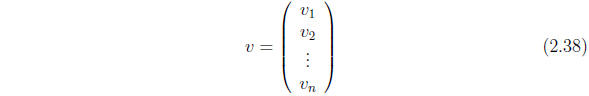
This has a compact expression in vector-matrix notation. Denote by v
the column vector

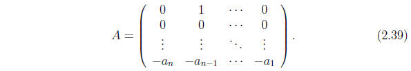
and by A the matrix

The inhomogeneous equation then has the expression

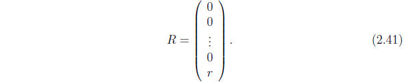
where v' is the vector made up of the corresponding derivatives of the components
of v, and

2.3.2 The general, linear system

The form of equation (2.40) looks, perhaps superficially, like that of the general
linear equation of first order encountered in the first chapter. It turns out
that the resemblance is more than superficial. Procedures from the abstract
(like the existence theorem) to the practical (like numerical solutions) are
unified by this formulation. Moreover, there is no need to restrict the first-order
systems of n equations that we consider to those derived from a single,
n-th order equation: we are free to consider the more general case of equation
(2.40) above wherein the matrix is an arbitrary matrix of
continuous functions, rather than one having the special companion-matrix
structure of equation (2.39) above, and the vector
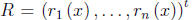
is an arbitrary vector of continuous functions rather than having the special
structure of equation (2.38).

Consider again the initial value-problem

where A(x) is an n×n matrix whose entries are continuous functions on an
interval I, R(x) is an n-component vector whose components are continuous
functions on I, is a point of I, and is an arbitrary vector of constants.
We again appeal to Chapter 6 for the basic conclusion:

Theorem 2.3.1 The initial-value problem (2.42) possesses a unique solution
on I.

This means that there is a vector v whose components are differentiable
functions of x on I, satisfies the differential equation v' = Av + R at each
point of I, and reduces to the given vector when x = . Again, as in the
case of the single equation of order n, it is useful to consider the homogeneous
case R ≡ 0 first.

The homogeneous system

The homogeneous system is written in our current vector notation as

If v and w are both vector solutions of this equation, so also is
for arbitrary constants α and β. This leads as before to the notion of linear
dependence of vector-valued functions on an interval I:

Definition 2.3.1 The k n-component vector functions are
said to be linearly dependent on the interval I if there exist k real numbers
, not all zero, such that

each point x of I. Otherwise they are said to be linearly independent.

In the theory of finite-dimensional vector spaces (like Rⁿ, for example),
a set of k n-component vectors is likewise said to be
linearly dependent if a relation holds for scalars
that are not all zero. The vectors above are functions
on an interval I and belong, for any particular value in I
to the n-dimensional vector space Rⁿ. But the requirement of linear
dependence is more stringent under the definition 2.3.1 than the
corresponding definition for a finite-dimensional vector space. The
relation

might hold for many values with a set of constants that are not all
zero (i.e., they may be linearly dependent as vectors in Rⁿ at those
points) without implying linear dependence on I: for this the equation
above would have to hold, for a fixed set of constants at
every point of I.

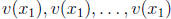
For example, consider the vector functions and
on the interval [−1, 1] (the superscript t stands for
transpose). It is easy to see that these are linearly independent under
the definition 2.3.1. However, if we set x = 0, each of them is the zero
vector and they are linearly dependent as vectors in R².

It is clear from the definition that, for any set of k functions
defined on the interval I, linear dependence on I implies linear dependence
on Rⁿ for each x ∈ I. Since linear independence is the negation of linear
dependence, we also have linear independence on Rⁿ at any point of I implies
linear independence on I.

We can easily infer the existence of a set of n linearly independent solutions
of the homogeneous equation: it suffices to choose them to be linearly
independent as vectors in Rⁿ at some point ∈ I. For example, we could
choose () = (1, 0, . . . , 0)^t to be the first unit vector,
to be the second unit vector, and so on. We now show that the solutions
of the homogeneous equation with these initial data
are linearly independent according to the definition 2.3.1. For suppose that,
for some value , the n vectors are linearly dependent
as vectors in Rⁿ. Then there are constants , not all zero,
such that

Using these constants, denote by v(x) the sum

It is a solution of the homogeneous equation vanishing at . But by the
uniqueness theorem it must vanish identically on I. This is not possible at
unless , a contradiction. Since could have been any
point of I, this shows that is linearly independent on Rⁿ at any point
of I and therefore, by the remark above, linearly independent on I. We have
proved the following theorem:

Theorem 2.3.2 Let each of the n-component vector functions satisfy
the homogeneous differential equation (2.43), and suppose that for some
∈ I the vectors are linearly independent as vectors in Rⁿ. Then
they are linearly independent on I.

As before, a set of linearly independent solutions of the homogeneous
equation is called a basis of solutions, and any solution of the homogeneous
equation can be written as a linear combination of them. If is a
basis of solutions, one can form the matrix

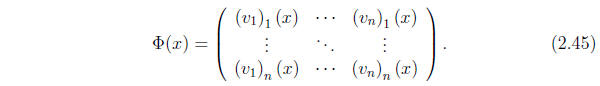
This matrix, sometimes called a fundamental matrix solution of equation
(2.43), and consisting of columns of a basis of vector-valued solutions, satisfies
the matrix version of the latter equation,

and is nonsingular at each point x of I. A useful version of this matrix is
that which reduces to the identity matrix E at a specified point . In terms
of this matrix, the solution v(x) of the homogeneous problem reducing to the
vector when x = is .

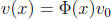The Inhomogeneous Solution

Return now to the inhomogeneous problem (2.42), and suppose that we have
solved the homogeneous problem and can form a fundamental matrix solution
. The variation-of-parameters formula has the structure ;
we leave it to the reader (problem 12 below) to work out the function w such
that this provides a solution of the inhomogeneous problem.

PROBLEM SET 2.3.1

1. Work out the Wronskian for the solutions found in Example 2.2.2. Referring
to Theorem 2.2.2, explain why the Wronskian is constant.

2. Same problem as the preceding for the solutions of Example 2.2.3.

3. Find a basis of solutions for the system u'''+u'' = 0. Calculate theWronskian
and check the result against Theorem 2.2.2 (equation 2.33).

4. Same as Problem 3 but for the equation

5. Write out the Wronskian W for three functions. Assuming that
they satisfy a third-order, linear, homogeneous differential equation, derive
the formula of Theorem 2.2.2.

6. The formula for the derivative of a determinant whose entries depend on a
variable x is

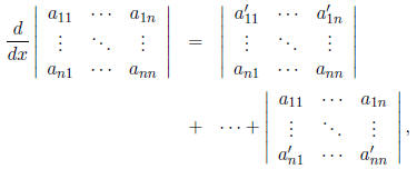
that is, it consists of n determinants, of which the first is obtained by differentiating
the entries in the top row and leaving the others unchanged, the
second by differentiating the entries of the second row and leaving the others
unchanged, etc. Using this and other, more familiar, rules for manipulating
determinants, prove the general version of Theorem 2.2.2. tex

7. For the operator Lu = u'''+u', find the most general solution of the equation
Lu = 1 (cf. Example 2.2.3).

8. For the operator of the preceding problem, obtain the influence function for
solving the inhomogeneous problem.

9. Carry out the uniqueness part of Theorem 2.2.1 if n=3.

10. Carry out the proof of Theorem 2.1.4 for the nth-order homogeneous problem.

11. Find the equivalent first-order system (that is, find the matrix A and the
vector R of equation (2.40)) for the second-order equation

12. In the general, inhomogenous system v' = A(x)v + R(x), choose to be a
fundamental matrix solution of the homogeneous problem that reduces to
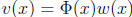
the identity at x = . Make the substitution v(x) = (x)w(x) to find a
particular integral v that vanishes at the point of I.

13. Let represent the determinant of an n×n matrix solution of equation
(2.46) above. Using the formula given in problem 6 above, show that
satisfies a first order equation

and express the function a(x) in terms of the entries of the matrix A.