Solution of the Equations

How do we know linear equations have solutions? Well, we can solve them by
algebra. For example:

17x + 4 = 1
17x = 1 − 4 = −3

We can do the same for many quadratic equations, using the quadratic formula:

If ax² + bx + c = 0, then

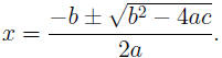
As long as the expression under the radical sign is not negative, we’ll get one or
two real-number solutions. (We’ll think more about what happens if it is negative
later.) It turns out there are similar, but longer, formulas for degree three, and
even degree four polynomials. But they seem to get harder and harder as the
degree gets larger, and last week we saw that there are some polynomials of
degree five and higher that are impossible to solve by an explicit formula. But we
can try another approach: Consider the polynomial equation 3x⁵ − 15x + 5 = 0
(One of the “impossible” equations featured last week.).

Figure 1. Graph of p(x) = 3x⁵ − 15x + 5

Its graph certainly appears to cross the x-axis in several places. And indeed
it does: We can calculate that p(0) = 5, p(1) = −7, and then apply the
Intermediate Value Theorem to conclude that its graph must cross the x-axis
somewhere in between:

Theorem. Let f be a continuous, real-valued function defined on a closed interval [a, b]. If y is any number between f(a) and f(b), then there is at least one c in [a, b] with f(c) = y.

If you take the time to understand what this theorem is saying, it might seem
obvious: to move continuously from f(a) to f(b), you need to pass through
each point in between. It is obvious. But the fact that it is both obvious and
true is deep, because it shows how closely the real number system models our
intuitive notions of continuity and connectedness. The statement would be false,
for instance, if we restricted attention only to rational numbers or integers.

What about other polynomials? If p is any polynomial of odd degree, we can
generalize the geometrically “obvious” thinking we saw above:

• If then for large x-values, p(x)
behaves much like its highest degree term: (Of course, the
meaning of “ ≈ ” is relative: the difference between p(x) and  a_nxⁿ is only
small compared to the size of p(x) itself.) Let’s assume a_n is positive from
now on, just for convenience.

• If a_n is positive, then, a_nxⁿ is positive when x is positive, and – because
n is odd – negative when x is negative.

• Thus for large positive x-values, p(x) is positive, and for large negative
x-values, p(x) is negative.

• So, by the Intermediate Value Theorem, a root exists somewhere between
these large negative and large positive x-values.

What about even degree polynomials? To take a simple case, let p(x) = x² −
2x + 2:

Figure 2. Graph of p(x) = x² − 2x + 2

As you can see, the parabola “goes upward” on both sides, and does not cross
the x-axis anywhere. But the quadratic formula does give us the two “solutions”
and Do they have a geometric interpretation terms
of intersecting graphs?

In fact, they do. The numbers are not real (in the sense of having
addresses where they live on the real number line). We can think of them as new
kinds of numbers, and if we visualize the reals as extending horizontally, then we
can pick one of the two (arbitrarily), call it i, call the other −i, and place them
vertically above and below the real number line along the y-axis.

Once i becomes a number, it has the same rights and duties to be added, subtracted,
multiplied, and divided as any of its “real” brethren do. Just as multiplication
by a positive number a sends a real number horizontally a times as far
from 0 as it used to be, the same operation with a real number b sends i vertically
b times further away. In this way, we label each point (0, b) along the y-axis with
the new number bi. Thus every “address” (a, b) in the xy plane becomes the
home of the so-called “complex number” a+bi. Moreover, we can add complex
numbers simply by adding their horizontal and vertical coordinates separately:

(a + bi) + (c + di) is defined as (a + c) + (b + d)i.

And we can multiply them, too, simply by treating i², whenever we see it, as −1.
We thus extend ordinary arithmetic with real numbers to the complex realm.

Just as the set of real numbers is often denoted R, we use C for the complex
numbers.

Now the fact that the two complex numbers and
appeared as roots of the polynomial equation x²−2x+2 = 0 means, algebraically,
that when we apply the extended arithmetic of the complex numbers to plug them
into the polynomial p, the result is 0. What about geometrically?

We graph a function f on the real line R using two copies of R which are
perpendicular to each other, intersect in a point, and together form a plane,
R2. Numbers on the first (horizontal) copy represent inputs, and numbers on
the second are outputs. Each point (x, y) which lies on the curve of a graph
corresponds to the function value f(x) = y. And the intersection of two curves
(like a graph and the x-axis) corresponds to a common solution to a pair of
equations.

Naturally, then, we would graph a function on the complex plane C using two
copies of C which are perpendicular, intersect in a point, and together form. . .a
what?

. . . Aye, there’s the rub. If we put two perpendicular planes together, we should
get a four-dimensional space, but humans have a tough time visualizing such a
thing. That’s where mathematicians come in.

Instead of a “curved line” in R², the graph of a complex-valued function will
consist of a “curved surface” in C². The fact that the quadratic formula gives
the two roots x = 1±i for the equation p(x) = 0 means that the curved surface
graph of p intersects the first copy of C in C² (the 2-dimensional counterpart to
the x-axis in the real case) in those two points.

Notice that, in this case, at least, jumping from the reals to the complex numbers
has insured that our even-degree polynomial has roots. Can we generalize that
argument using the intermediate value theorem to show that every polynomial,
of odd or even degree, has a root among the complex numbers? Let’s try. Our
first step is a nice bit of geometry: We can rewrite the “addresses” of complex
numbers using polar coordinates:

We label points in the plane by indicating the direction (in terms of an angle
measured from the x-axis) and distance from the origin, rather than by their horizontal
and vertical displacements from 0. It isn’t too hard to calculate formulas
for the translation in each direction:

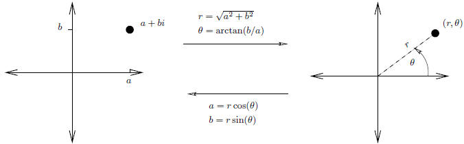
The corresponding re-labeling of complex numbers has some nice properties:

• The number whose polar coordinates are (r, θ ) is actually equal to re^iθ .
(Yes, that’s the familiar e ≈ 2.71828 from calculus. In the name of equal
rights for complex numbers, we’re extending our familiar exponentiation
function to allow for imaginary exponents.)

• Using the rules for multiplying exponentials, we have

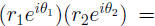
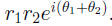
• Thus to get the polar-coordinate “address” of the product
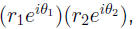
we multiply the distances from 0 and ADD the angles.

In particular, we can geometrically understand the function p(x) = xⁿ by noting
that

It stretches distances from 0, and multiplies angles by n. For instance, p(x) = x²
will carry each point on the unit circle to a corresponding point with twice the
angle, and hence wrap the circle around itself twice. And it would wrap the
radius 2 circle twice around the radius 4 circle, the radius 3 circle twice around
the radius 9 circle, and so forth. . . . So in general,

The function p(x) = xn wraps the whole complex plane n times around itself, and stretches it radially via

Now here is the basic principle which generalizes the Intermediate Value Theorem:

Theorem. Let f be a continuous, complex-valued function defined on a closed disk D. If f maps the boundary of the disk n > 0 times around the boundary of another disk D0, and y is any point in the interior of D0, then there is at least one c in D with f(c) = y

This may not seem quite as obvious as the Intermediate Value Theorem itself. But
it reflects how closely the complex number system models our intuitive notions
of continuity and two-dimensional connectedness: If you were to stretch the
boundary of a rubber disk around another disk, with no rips or punctures, it
would have to cover every point in the second disk.

Now we are in a position to understand the first version (the regular-strength
version, we might say) of the